
![]() By Mark Stetz,* P.E. CMVP
By Mark Stetz,* P.E. CMVP
When developing regression models for Option B or C methods, M&V practitioners often place too much emphasis on developing models with high r2 values and too little on minimizing uncertainty. A high r2 value does not guarantee that a particular model can (or should) be used; having a low r2 value does not necessarily preclude a model from being used.
Both IPMVP and ASHRAE Guideline 14 define the acceptable level of savings uncertainty – the most important criterion by which a model’s validity and usefulness should be assessed. This paper describes the pitfalls of focusing on maximizing r2, shows the importance of CvRMSE in assessing savings uncertainty, and presents example Option C models used to evaluate savings in real performance contracts where the results may be counter-intuitive to many.
Abbreviations

Background
The fundamental premise of measurement & verification is to compare current energy use to the estimated energy use under current operating conditions - what would have happened absent the energy-efficiency upgrade. For Option C and many Option B approaches, linear regression modeling is the workhorse method of creating adjusted baselines that reflect current conditions. Developing reliable and useful models is therefore critical to establishing a robust and repeatable M&V procedure.
Software products such as Microsoft ExcelTM allow practitioners to develop ad hoc linear regression models of complexity limited only by user skill. The graphing function and linear regression model tool make it easy to develop polynomial and multivariate regression models.
The selection of which model is the “best” to use is often made based on which equation form and/or variable set has the highest r2. But like so many things in life, there are answers that are fast, simple, and wrong. Selecting the model with the highest r2 is often not the “best” model to use.
The correlation coefficient r2 quantifies the extent to which the independent variable(s) drives the dependent variable but little else. Correlation implies - but does not prove - causality. The model needs to represent the underlying physical relationship between the variables. For example, a regression model of monthly heating load on a building may have a higher r2 when a quadratic model is used instead of a linear model, but there is no thermodynamic principle that explains why a linear heating load might behave in a non-linear fashion. On the other hand, fan power as a function of speed should be modeled with a third-order polynomial or power-law model because the physics support it.
Common “fixes” to low r2 values include adding independent variables that may have little relationship to the dependent variable being modeled, or using an equation form that defies physics. This author has seen others develop regression models of hourly AC energy use using six variables that included the current temperature, current temperature squared, the temperature one and two hours prior, current wet bulb temperature, and the sine of the day of the week. The temptation to improve r2 is great but the potential for abuse is high.
Linear regression modeling is an exceptionally powerful tool provided the following points are considered:
- The model represents the physical relationship between the independent and dependent variables. Don’t use polynomials or power laws to model linear systems.
- The independent variables need to be independent of one another. For example, Tdry bulb and Twet bulb are not independent – they are highly correlated. Use Tdry bulb and Tdew point instead. Or better yet, use enthalpy H. And please don’t model kW/ton as a function of tons as the tons cannot simultaneously an independent and dependent variable.
- When using multivariate models, use at least three to five time as many data points as the number of independent variables. Then reject variables with |t| < 2 and develop a new model.
- When it comes to adding additional variables or using polynomials, remember: just because you can doesn’t mean you should.
A more thorough discussion of developing and evaluating regression models for M&V purposes can be found in Bonneville Power Administration’s Regression for M&V: Reference Guide.
Savings Uncertainty
Ultimately a regression model is useful only if the adjusted baseline it creates results in savings uncertainty that is within acceptable limits. ASHRAE Guideline 14 requires that the savings uncertainty be less than 50% of the annual savings at 68% confidence. IPMVP recommends the savings be more than twice the standard error of the baseline value. Six of one, half a dozen of the other. These statements are identical and provide guidance on what constitutes an acceptable level of savings uncertainty.
Uncertainty Assessment for IPMVP (2018) defines how to calculate the overall savings uncertainty for a given regression model when using monthly utility bill data. Setting t to 1 (68% confidence level) and ignoring the baseline adjustment factor, equation 58 reduces to:
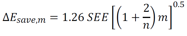
Where m and n are the number of periods in the post-retrofit and baseline periods respectively. ASHRAE’s Guideline 14 offers a similar equation to define the uncertainty, except in relative units. Guideline 14 Equation 4-8 (ignoring t) is:
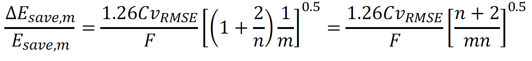
Here, m and n have the same meaning while F connotes the relative savings fraction. The derivation of these two equations is discussed in Uncertainty of “Measured” Energy Savings from Statistical Baseline Models.
To calculate one form from the other, recall that:
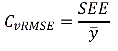
This is a useful relationship to remember when evaluating regression models in a spreadsheet where SEE is provided but CvRMSE is not.
Guideline 14’s equation 4-8 shows that the uncertainty is related to CvRMSE and savings fraction F but NOT the regression model coefficient r2. To reduce uncertainty to acceptable levels, CvRMSE needs to be low and F high. (Increasing the number of months in the baseline period has only a minor influence.) This relationship can be easily evaluated over a range of conditions to illustrate the sensitivity of uncertainty to the savings fraction F and CvRMSEs.
In the following table, the baseline and post-retrofit periods are assumed to be one year each (m=n=12). This shows that the greater the CvRMSE, the greater the savings fraction F needs to be to adhere to ASHRAE / IPMVP guidance. Combinations with uncertainties exceeding acceptable levels are shaded in grey. The rule-of-thumb that savings F should be at least 20% of the baseline and CvRMSE < 0.2 yields a result with an acceptable level of uncertainty. This is not a coincidence.
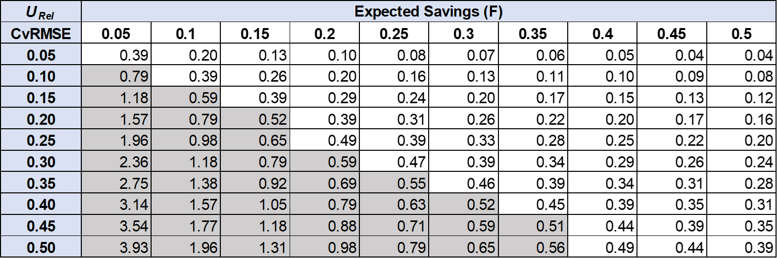
When savings are < 15%, acceptable uncertainty can be achieved only for models that have very low CvRMSE values.
Application of CvRMSE : Example 1
To demonstrate the value of CvRMSE as an evaluation metric, consider a real-world example. An ESCO is proposing upgrades at a bundle of mosques in Riyadh, Saudi Arabia. Mosques are simple structures that can be treated as single-zone concrete boxes containing only lights and AC equipment. Operating schedule is well defined and consistent – mosques are used five times a day, 365 days per year. The proposed ESMs are lighting upgrades, AC scheduling that coincides with prayer times, and a limited number of AC replacements to higher EER units. As expected, energy consumption is dominated by air-conditioning in this hot dry climate (Zone 0B), with 70% of the total energy use allocated to AC.
Given the high degree of correlation of monthly energy consumption to cooling degree-days, the ESCO has proposed Option C as the M&V approach. Let’s look at the regression model statistics to see how the r2, CvRMSE, savings fraction F, and relative uncertainty URel (@ 68% confidence) align. In the following table, the average r2 exceeds 0.9 indicating a very high degree of correlation between CDD and energy use across the population. Despite the very high correlation, the average savings uncertainty for each individual mosque is just under 30%. While 18 mosques have individual uncertainties adhering to ASHRAE / IPMVP recommendations, the uncertainties are higher than the 20% uncertainty at 80% confidence criteria commonly used for other purposes.
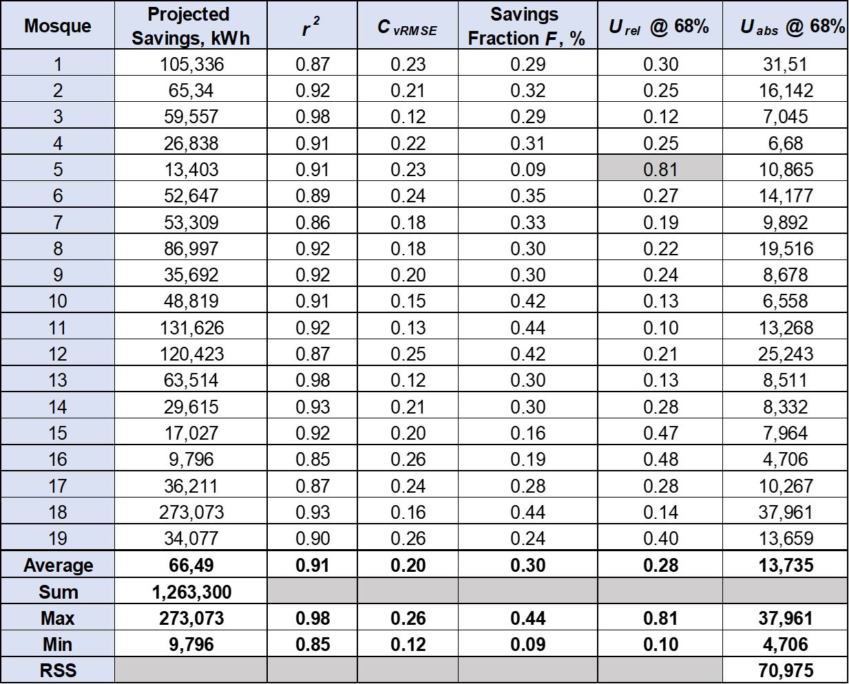
The uncertainty for mosque #5 of 81% (in grey) does not meet IPMVP / ASHRAE recommendations in part due to its high – but not the highest – CvRMSE. The large uncertainty is really caused by the low expected savings F of 9%. If this were the only mosque in the project, we would reject Option C as a viable M&V approach because the uncertainty is too great relative to the expected savings.
The regulatory body overseeing ESCO projects in Saudi Arabia wants the savings reported with an uncertainty of 10% at 90% confidence – eight times more stringent than ASHRAE / IPMVP recommendations! To see if this is achievable, recall that the overall uncertainty is found by summing the individual uncertainties in quadrature.
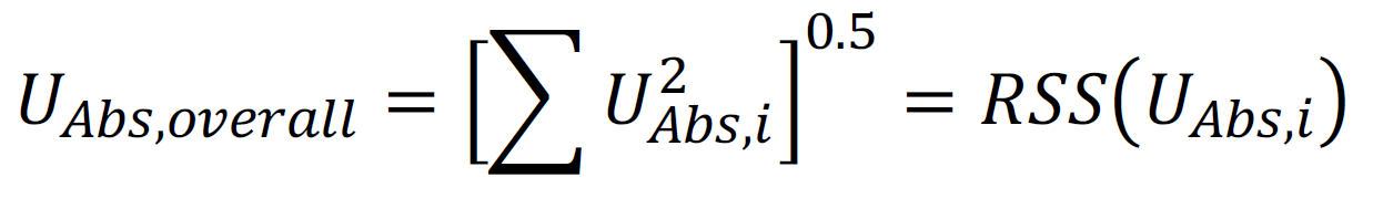
In this case, the overall uncertainty UAbs (at 68% confidence) is the root of the sum of the squares (RSS) of the individual uncertainties across 19 mosques: 70,975 kWh. To calculate the relative uncertainty URel, divide this value by the sum of expected savings: 1,263,300 kWh. To express this result at a 90% confidence level, multiply by t for the relevant degrees of freedom (d.f.= 18):

The desired savings uncertainty criteria has been met for the overall project by virtue of the power of the ‘portfolio effect’ whereby savings increase linearly while uncertainties increase to the one-half power. Whether the choice of 10% uncertainty at 90% confidence is appropriate for either individual or bundled projects is a different topic of discussion.
Application of CvRMSE : Example 2
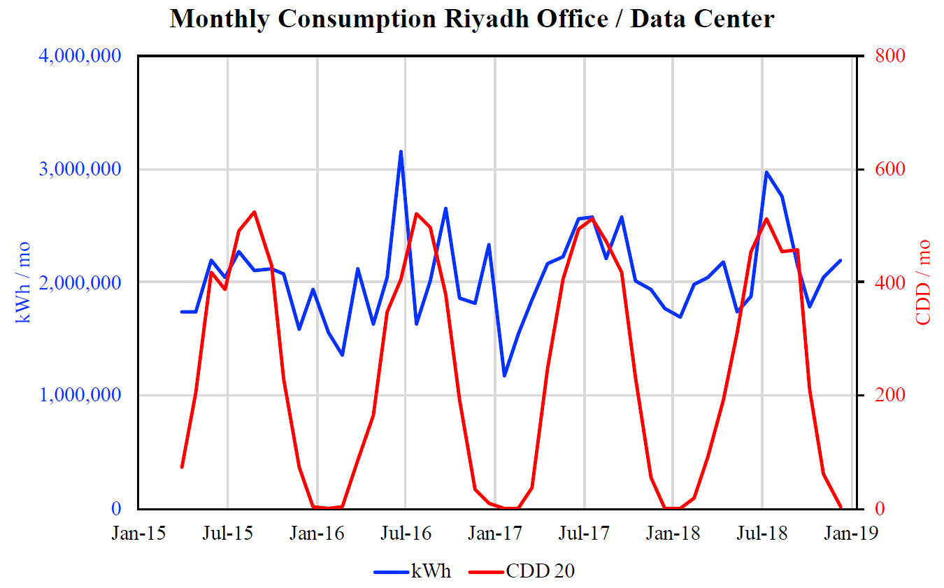
Consider a different scenario where r2 is lower than we might normally expect to see an Option C regression model used. This too is a project in Riyadh, Saudi Arabia, but it is an office complex with a load dominated by a large data center. This dilutes the weather-driven cooling since the data center is a large 24/7 load. The following time-series chart shows that while the monthly consumption varies, it does not appear highly correlated to cooling loads:
The scatter plot and regression model support that intuitive conclusion:
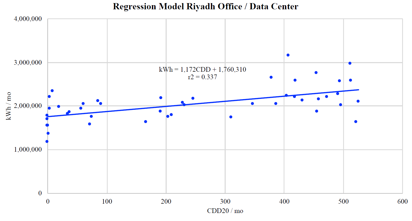
In this case, the r2 is only 0.38 – far below what would normally be considered acceptable. Per Statistics and Data Analysis: An Introduction, this indicates that the regression model is statistically significant at p=0.01 (n=46). The relationship between energy use and weather is weak but present.
The more important finding is that the near-constant load reduces the CvRMSE to only 0.16, which is a good indicator of the overall uncertainty that might be expected. Projected savings F are 30% of the baseline. Using the ASHRAE uncertainty equation and 46 months of baseline data yields an expected savings uncertainty of 20% (at 68% confidence) – well within the recommended limit. From the perspective of the country’s regulatory body, this is 34% at a 90% confidence level which exceeds their 10% target savings uncertainty by more than a factor of three.
Despite the initial impression that Option C could not be used due to the low r2, a more thorough uncertainty analysis shows that the low CvRMSE and high savings fraction F result in a case where Option C can be justified.
If Option C is the desired approach but one is uncomfortable using a regression model, similar results could be obtained by taking the average monthly consumption to establish the baseline. The average monthly consumption has a Cv of 0.19 – only slightly greater than the CvRMSE of 0.16. Using the average monthly value as the baseline would introduce slightly more uncertainty into the savings estimates while eliminating any argument over the r2 or suitability of the regression model generally. From a reporting perspective, this will introduce a trend in the monthly reported savings with lower values in the summer and higher in the winter. One way to minimize this trend is to average the savings by month (if n > 12) and use that as the baseline. The annual results will be the same, but the savings trend will be more reflective of the ‘actual’ savings.
Conclusion
When developing regression models, there is a strong tendency to focus on the correlation coefficient r2 to the exclusion of all else. It is tempting to use inappropriate model forms and add irrelevant variables to a regression model hoping to eke out a slight increase in r2 value. This applies to models used for both Option B and C. As M&V practitioners, we should be taking our guidance from IPMVP and ASHRAE Guideline 14 that remind us our real goal is to minimize the uncertainty in the reported savings. When looking at the underlying mathematics, r2 does not drive savings uncertainty; CvRMSE and savings fraction F do.
In this paper, we have examined a case where multiple buildings have very high r2 values but only modest CvRMSE values. Absent an uncertainty analysis, we would accept the models as viable without assurance that the resultant savings uncertainty meets established criteria. Fortunately, they do – in 18 of 19 cases. However, the individual site uncertainty is higher than we might otherwise assume based on r2 values alone. The uncertainty is significantly reduced when considered in aggregate. This is good news for Program Administrators and Managers overseeing portfolios of projects.
We also looked at a single case where one might reject Option C as a viable M&V approach due to a low r2 value. Closer examination shows that the CvRMSE is sufficiently low and the savings fraction F sufficiently high such that the savings uncertainty is within acceptable IPMVP / ASHRAE G-14 recommendations despite the low r2 value.
The lesson here is not to jump to conclusions about whether a regression model can be used for any particular application based solely on r2. The correlation coefficient describes the strength of the relationship between the independent variable(s) and the dependent variable – and says nothing about the savings uncertainty that results from the model. When evaluating utility bills or logger results, listen to what the data is trying to tell you: sometimes there just isn’t a strong or quantifiable driving variable(s) present and no amount of additional variables or convoluted equation forms will change that. Stochasticism – like entropy – is always present and cannot be wished away. But we have the tools to evaluate whether our crude models are in fact useful if only we would learn to use them.
REFERENCES
Regression for M&V: Reference Guide
Bonneville Power Administration
Version 2.0 July 2018
Guideline 14-2014: Measurement of Energy, Demand, and Water Savings
ASHRAE
Atlanta, GA 2014
Statistics and Uncertainty for IPMVP
International Performance Measurement and Verification Protocol
2014
Uncertainty of “Measured” Energy Savings from Statistical Baseline Models
T. Agami Reddy, Ph.D., P.E. David E. Claridge, Ph.D., P.E.,
HVAC & R Research 2000
Uncertainty Assessment For IPMVP
International Performance Measurement and Verification Protocol
2018
Statistics and Data Analysis: An Introduction
Siegel, A.F.
John Wiley & Sons. New York, NY 1988

(*) Mark Stetz, P.E. CMVP is the founder and owner of Stetz Consulting LLC located in Colorado Springs, CO, USA. He has supported performance contracting including the US DOE FEMP’s ESPC program throughout much of his twenty-plus year career. He is currently working with the super-ESCO Tarshid (tarshid.com.sa) in Riyadh, Saudi Arabia as their M&V specialist. Stetz Consulting can be reached at www.stetzconsulting.com or mark@stetzconsulting.com.
![]()