
![]() By Anna Kelly** and Craig Sinnamon***
By Anna Kelly** and Craig Sinnamon***
ABSTRACT - ComEd’s Virtual Commissioning program relies on whole-building analysis and identifies savings as low as 3% of facility consumption. Utility program requirements frequently cite IPMVP Option C when requiring that whole building modeling should only be used to detect savings greater than 10% of consumption. There is a disconnect between requirements citing IPMVP and what a deeper reading of the protocol can clarify for the user.
Using IPMVP Option C methods for detecting savings <10%, we analyze daily and hourly energy efficiency projects and compare the differences between the methods and models used to generate those savings. The results demonstrate that it is possible for models to identify savings as low as 3% of facility consumption. Hourly models detect savings at the extremely low savings up to 6% and daily models perform equally well at 7% and higher.
IPMVP Option C guidelines, as well as previous ASHRAE guidelines, were written in 2002, and consequently, do not address advanced applications. The American Recovery and Reinvestment Act of 2009 (ARRA) however, provided over $3B for Smart Grid Investments and AMI deployment across the United States. At the same time, EVO’s IPMVP Committee has stated they are currently working on providing more detailed guidelines for the next major revision upcoming in 2021. The original IPMVP Option C was released prior to the advent of AMI data. Although it has been updated several times, utility programs across the US and Canada are continuing to default to the original 2002 version of IPMVP when evaluating projects assessed using whole building modeling.
Whole building regression modeling is being used by more programs to save program delivery costs and to move away from deemed savings values based on engineering calculations. To enable more programs to use interval data and find savings, energy efficiency program administrators and implementers need to be able to deploy more cost-effective programs. Allowing projects using IPMVP to seek out projects and claim savings that are lower than 10% of whole facility consumption will open up an entire new segment of previously untouched energy savings.
Introduction
Technology is changing at a rapid pace. Throughout history, regulators and measurement and verification (M&V) experts have worked to improve their methods and regulations to reflect the true nature of the technologies that they impact. Although the rate of technological advancement is changing rapidly, the shape of it is not. Innovation and adoption of new technologies follow an S curve. See Figure 1 for the US household adoption of the automobile, as well as in household adoption of electric power and radio. The S curve starts slow, with a small percentage of the population adopting a new technology first as innovators, with eventual long-term adoption by the vast majority of the population.
Figure 1. S Curves of U.S. household technology adoption 1900-2020 Source: Ritchie and Roser 2019
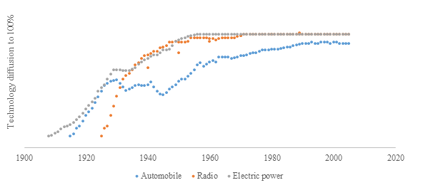
This curve has been seen time and time again throughout history with almost all technologies. However, Figure 2 shows that the speed at which the curve is changing has been accelerating dramatically in the modern era, with widespread societal adoption of new technologies not happening over a span of 80-100 years, but rather in a single decade. Rather than the slow S curve of adopting running water, electric power, and automobiles, modern technologies are adopted at a nearly vertical curve from the day of market introduction.
Figure 2. S Curves U.S. household modern technology adoption 1950-2020 Source: Ritchie and Roser 2019
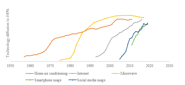
The increasing speed of technological adoption poses challenges for regulators. With automobile adoption, the nation had 40 years to create the first set of regulations for the first half of society that was adoption cars. Looking at air conditioning, even though the timeline is compressed, there was still a 20 year gap before 50% adoption. But the technologies introduced in the last half century have had widespread adoption within a decade of introduction. That speed does not leave room for regulations and policy documents to capture the complexity of the technology at release. The rapid adoption of new technologies has been challenging for policymakers across all segments, and that is also true for the energy industry. Energy efficiency was slowly becoming a well-regulated industry by the early 2000s. The International Performance Measurement and Verification Protocols (IPMVP) were adopted across the world by the end of the 2000s, and those, among other protocols, provided frameworks with which efficiency program administrators, implementers, and evaluators could reliably calculate avoided energy use from energy efficiency projects.
In 2009, in order to stimulate the economy and recover from the 2008 recession, the American Reinvestment and Recovery Act (ARRA) was passed and provided $787 billion in funding to sectors across the US, with $43 billion dollars of that funneling into the energy industry. Of that $43b, $3b was invested into Smart Grid Investments and Advanced Metering Infrastructure (AMI) deployment across the country. This new technology provided a wealth of brand-new data that utilities, energy efficiency programs, implementers, and evaluators could use to identify deeper savings and provide more granular analysis of existing projects. However, utilities and other stakeholders quickly learned that actually using AMI data was going to be far more challenging than initially anticipated. Among privacy concerns, connectivity issues, and reliability concerns, another issue slowly emerged. There were data scientists and econometricians skilled enough and willing to use the data, but the protocols that had been written in the early 2000s to support evaluation, measurement, and verification (EM&V) activities were all designed to support analysis using monthly billing data. This would not have been a major problem, if not for the slow diffusion of the protocols into program requirements documentation and rulemaking proceedings to mandate the use of these protocols as written, namely IPMVP Option C (whole building modeling).
Requirements for Whole Building Modeling
Whole building regression modeling started being used in earnest in the first strategic energy management (SEM) programs starting around 2009. At that time the models were typically specified as energy (kWh) as a function of outside air temperature either expressed as a mean or cooling degree days and heating degree days (CDD and HDD), production variables (e.g. # of widgets produced, lbs of widgets produced, lbs of waste widgets produced, dollar value of sales, etc.), occupancy indicators, and dates of energy efficiency projects. In the beginning, this was done with monthly billing data entered in to a spreadsheet and then regressed in an attempt to identify the extent to which the energy efficiency projects were influencing facility kWh while controlling for the other drivers of consumption. Early modelling was fraught with complications, inability to replicate, and an overall industry skepticism that the estimated savings values had the same legitimacy as deemed values. Even though programs using regression modeling were new, the idea was not. The industry legitimized the use of regression modeling by adopting existing protocols.
IPMVP
The IPMVP has been updated with major releases every 5 years and clarifying documents released as needed in the interim. The original was the North American Measurement and Verification Protocol released in 1996. It was renamed and reissued the next year after widespread international interest. There have been four official updates to the protocol in the time since the initial release, with each one accounting for more modern technology and energy efficiency program types. In 2014, the first IPMVP Core Concepts was released. The Core Concepts are abridged versions of IPMVP that are split up into individual protocol documents that allow for more frequent updating and more flexible content. The Core Concepts were revised in 2016, and EVO is currently working to release an updated version again in 2021.
With regards to the 10% savings threshold, IPMVP has updated the language several times. The 2002 Volume 1 says, “Typically savings should be more than 10% of the base year energy use if they are to be separated from the noise in base year data” (USDOE 2002). The 2012 update approached the minimum savings value from a different direction, saying “Typically savings should exceed 10% of the baseline energy if you expect to confidently discriminate the savings from the baseline data when the reporting period is shorter than two years.” (EVO 2012). The 2016 Core Concepts was even more specific in its advancement,
“As a rule of thumb, if only monthly billing data are available for energy consumption and demand, savings typically must exceed 10% of the baseline period energy if you expect to confidently discriminate the savings from the unexplained variations in the baseline data.
When short-time interval energy consumption data are available, the number of data points is much greater, and advanced mathematical modeling may be more accurate than the linear models used for monthly analysis. Consequently, methods using short-time interval data and advanced algorithms may be able to verify expected savings that are lower than 10% of annual energy consumption. In either case, an assessment of baseline model accuracy with expected savings and monitoring period duration is required.” (EVO 2016)
Reading the IPMVP updates released over time show that EVO is regularly updating the language and opening pathways for programs to detect savings that are under 10% of facility savings. IPMVP’s Snapshot on AM&V and IPMVP M&V Issues and Examples are two recent publications that clarify this rule of thumb.
IPMVP M&V Issues and Examples says:
- Section 3 under ‘Method Selection’ includes a ‘rule of thumb’ of 5% for Option C using frequent energy data and 10% for monthly data; and
- Section 4.3 is “Advanced M&V Methods” focused on using interval meter data with Option C.
IPMVP’s Snapshot on AM&V provides further clarity intended to help clarify this and other issues until a major update could be released. The upcoming IPMVP Application Guide on Advanced M&V Methods (end of 2020) will further attempt to eliminate confusion on the issue, and the new Core Concepts will be out in 2021.1 However, the issue of the 10% rule of thumb turning into a requirement is not seen only in IPMVP. There are protocols other than the IPMVP that also reference the 10% rule, even in the most recent updates.
ASHRAE 14-2014 says “Compliance requires site savings to be in excess of 10% of facility energy consumption... “expected savings shall exceed 10% of measured whole- building (or relevant submetered portion of whole-building) energy use or demand” with daily data as the minimum granularity permitted (ASHRAE 2014). Bonneville Power Administration’s Regression for M&V Protocol is one that does not mentioned a minimum savings threshold at all (Research Into Action 2012). There are several other common protocols used in M&V for this industry, but the ones mentioned above have the most relevance to the current discussion.
Legislation and Program Rules Referencing IPMVP
As of early 2020, language referencing compliance or adherence to IPMVP Option C is deeply integrated in program management plans, legislation, and utility M&V guidelines. The guidelines nearly always reference the original IPMVP in full: IPMVP: International Performance Measurement and Verification Protocol: Concepts and Options for Determining Energy and Water Savings, Volume 1 with no reference to updates to the protocol such as the 2016 Core Concepts or the IPMVP Generally Accepted M&V Principles (EVO 2018).
This can lead to considerably confusion for program implementers and administrators designing compliant programs. Consider a new program attempting to use meter data to run regression modeling in the state of California. The designers of this program may be discouraged from launching because the new Rulebook released January 2020 uses the 2007 IPMVP language and mandates extra steps, justifications, and calculations for programs targeting savings less than 10% of facility consumption (CPUC 2020). Lawrence Berkeley National Labs released an update technical guidance document to assist programs in developing their M&V plans that references the Core Concepts, rather than simply saying “IPMVP Option C,” but that level of detail is by far an exception in current guidelines and program rules for programs hoping to use whole building modeling (LBNL 2018).
As a result of the decades long expectation of monthly data, the industry has little experience looking for savings smaller than 10%. Compounding the issue is the lack data showing the differences in modeling at a daily or hourly level. The next section will outline the methodology that the authors used to explain energy consumption using daily and hourly regression models, followed by discussion on the results.
The Study
This remainder of this paper compares hourly and daily modeling methods using the same data set of 192 non-residential facilities. The purpose of this comparison is to identify the acceptability of models using high granularity inputs to measure savings. In particular, the analysis will focus on identifying savings lower than 10% of facility consumption (e.g. a facility with 100,000 kWh annual consumption saving 10,000 kWh or fewer from an energy-efficiency intervention.)
Basic Methodology
Daily Models
Daily electricity consumption is modeled as,
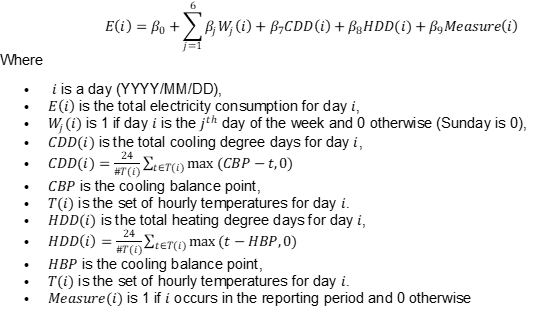
Note: This daily equation is linear except for the dependence of the heating and cooling balance points. These balance points are selected by fitting models for all pairs of integer grid points (between 50 and 75 degrees Fahrenheit) and selecting those that produce the model with the highest adjusted R2.
Hourly Models
Hourly electric consumption is modeled as,
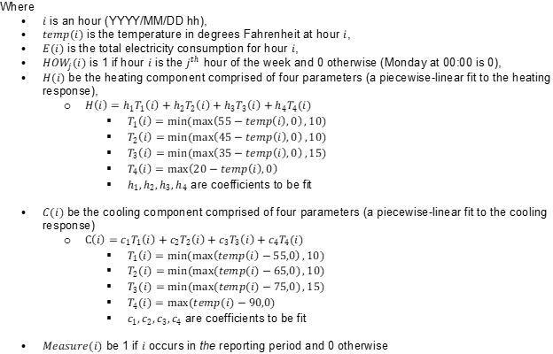
All models must pass basic model fitness requirements.2
- NMBE < 0.5% 3
- CV(RMSE) < 25%
- Savings Uncertainty < 50% at 68% confidence
Definitions:
- CV(RMSE) (coefficient of variation of root mean squared error): CV(RMSE) is a key metric for model evaluation and an indicator of random error. Calculated as the RMSE divided by the average energy consumption, it quantifies the typical prediction error as a percentage (expressed as a percentage, lower is better). CV(RMSE) reports the model’s ability to predict the energy use.
- NMBE (net mean bias error): NMBE measures bias of the predicted consumption relative to the actual consumption.
- Fractional Savings Uncertainty: Metric that shows the impact of model and prediction error on the reliability of the savings estimate relative to the savings of the model. Currently subject to much ongoing research and testing on how to best estimate savings uncertainty with high granularity data (PG&E 2018; Boonekamp 2006; Touzani et al. 2019; Kissock and Eger 2008; Sever et al. 2011).
Results
The 192 non-residential sites were run using an hourly and a daily model specification to compare the differences between the models. The results section has daily results first, then hourly, and then a discussion about the implications of this work.
Daily
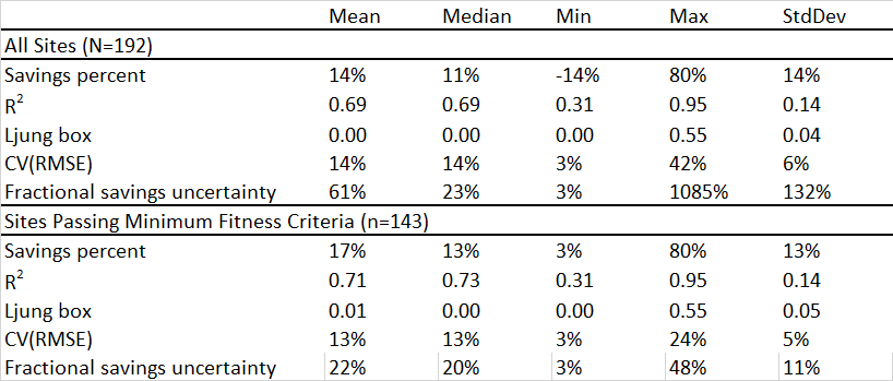
The daily model takes half hour data and aggregates it into 24 one-hour periods. The analysis was run on the same 192 sites for both daily and hourly. Table 1 shows basic summary statistics on the outcome of the daily model for these sites. The table is split into two sections: all sites, and sites that passed minimum fitness criteria (referenced in Basic Methodology). Sites that pass with minimum fitness criteria have an average of 17% savings, with the mean value dragged upwards by the maximum savings value of 80% of facility consumption. One interesting factor of note is the low R2 that is found in the passing models. Although the mean is .71, the minimum was .31. As referenced in Footnote 1, R2 should not be used to determine if a model should be accepted or not. The Ljung Box is a measure of autocorrelation, which is used as a test to identify the extent to which the consumption data is in violation of the regression assumptions on the distribution of noise (low values are good, a high value is typically above 10 with this type of consumption data).
Table 1. Daily model summary
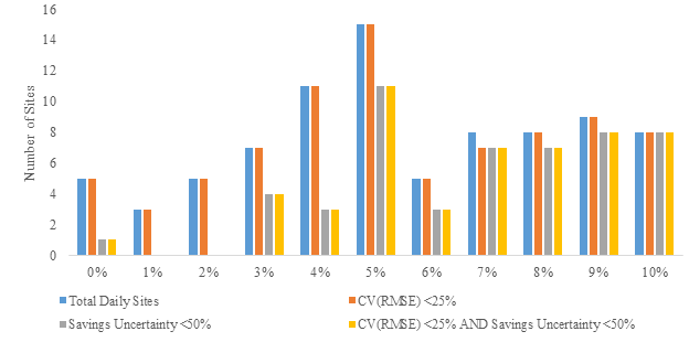
Of the 192 total sites, 43% have savings that fall under 10% of facility consumption. When split into bins showing savings less than 10% as a percent of facility consumption, the daily model has the highest proportion of passing sites starting at 5% of facility consumption. Figure 3 shows the total number of sites with recorded savings in the 0-10% range as well as the sites that pass the two varying fitness metrics in each combination. Eight of eighty-four sites with savings <10% pass in the <5% range, forty-four pass in the 5%-10% range, and 32% do not meet the minimum fitness criteria. All but one of the sites have a CV(RMSE) under 25%.
Figure 3. Comparison of daily sites with savings values at or below 10% of total facility consumption
Hourly
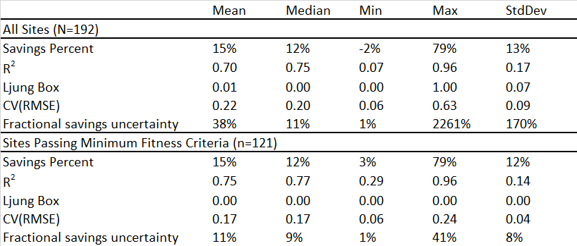
The hourly model was run using the same sites as the daily model. Table 2 shows that the hourly model provides similar savings estimates to the daily model, especially among those sites that pass the minimum fitness criteria. The CV(RMSE) reported from the hourly model tracks higher than that of the daily model, and the savings uncertainty is lower.
Table 2. Hourly model summary
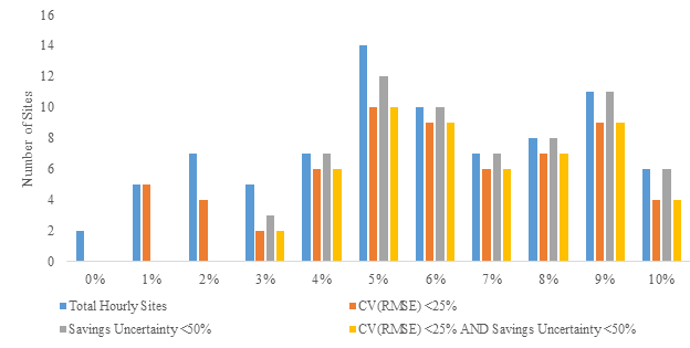
When split into bins showing savings less than 10% as a percent of facility consumption, the hourly model, like the daily model, has the highest proportion of passing sites starting at 5% of facility consumption. Figure 4 shows the total number of sites with recorded savings in the 0-10% range as well as the sites that pass the two varying fitness metrics in each combination. Eight of eighty-four sites with savings <10% pass in the <5% range, forty-five pass in the 5%-10% range, and 35% do not meet the minimum fitness criteria. Sixty-two sites have a CV(RMSE) under 25%.
Figure 4. Comparison of hourly sites with savings values at or below 10% of total facility consumption
Discussion
Although the daily model and the hourly model can identify savings to approximately the same level of granularity, there are definite pros and cons to each approach. Figure 5 shows a comparison between hourly and daily models that pass basic model fitness requirements at sub 10% facility savings. For the most part, detecting savings under 3% is not common or consistent. In other simulations run by the authors, the same results have been noticed where savings <3% are not readily detectable. However, above 3% of facility savings, the models begin passing basic model fitness requirements.
Figure 5. Daily and hourly model comparison for <10% facility savings
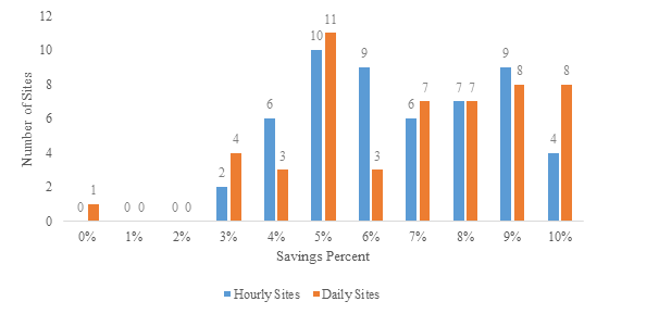
In the sample of sites used in this analysis, more of the hourly sites pass fitness criteria than daily sites in the 4-6% of facility consumption range. Daily sites pass more frequently after hitting reaching 7% of facility savings. Table 3 shows the distribution of savings under 10% for the hourly and daily models. This suggests that hourly modeling is better able to detect savings at a lower level than daily models, but more research is needed.
Table 3. Savings bin with percent of sites passing minimum fitness criteria

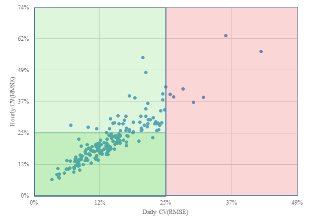
Figure 6 provides a visual overview of the individual sites in the sample and their hourly and daily CV(RMSEs). The light green box on the left hand side of the chart show the acceptability range for the daily CV(RMSE), and the dark green box in the lower left quadrant show the area where both the daily and the hourly models are within the acceptable range. It is noticeable that many more of the sites fall within the daily CV(RMSE) acceptability range, where comparably few of the hourly sites do.
Figure 6. Daily and hourly CV(RMSE) comparison
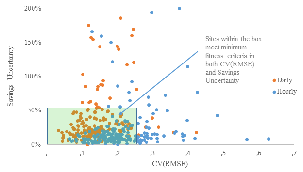
Savings uncertainty is likely underestimated by the hourly model, as shown in Figure 7 (LBNL 2018). The cluster of hourly values shows a significantly lower savings uncertainty than the daily values, which show a smaller CV(RMSE) but more variation in the calculated savings uncertainty.
Figure 7. Savings uncertainty and CV(RMSE) for daily and hourly models
Specifically, it is a challenge to calculate savings uncertainty with accuracy when modeling with hourly resolution. The method used in this analysis attempts to take into account the dependence between variables due to the use of a single model for baseline and reporting periods. Savings uncertainty is based on an estimate of the standard error of the savings. An estimate of the standard error will be based on the results of the regression model for the energy consumption. The more ill-behaved the noise term in the regression model, the more bias is to be expected in the regression results. In particular, when using low resolution interval data (hourly) there will be more autocorrelation in the noise term than when using higher resolution interval data (daily). This leads to more bias in the model coefficients, and more autocorrelation in model residuals leading to greater challenge in estimating the standard error in the savings in an unbiased way (EVO 2018). LBNL (2018), demonstrates that the ASHRAE savings uncertainty calculation is more likely to understate the uncertainty in a prediction when using an hourly model as opposed to a daily model.
Methodology regarding uncertainty calculations is not within scope of this paper, but interested parties may use the references section to get a starting point on the differences in calculation methods used by various industry actors.
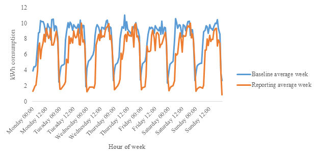
The daily model may provide slightly more accurate fitness criteria, but there is a level of understanding with the hourly model that increases its usefulness to program actors and utilities. See Figure 8 for a plot of an average week’s energy consumption with no heating or cooling response using the hourly model. At this site, the facility implemented a new lighting schedule introducing a complete overnight shutdown as well as a delayed startup to their facilities in the morning. This level of granularity provides value for the program participant to be able to truly visualize the intervention that they implemented, and for the utility when they are attempting to provide different incentives based on time of use metrics.
Figure 8. Average week using hourly model
Policy and Program Implications
The data analyzed in this report suggest that it is appropriate to use IPMVP Option C methodology to identify savings under 10% for whole building modeling when using daily or hourly level source data. The industry rule of thumb of a 10% minimum should be changed to an industry rule of thumb that we carefully read all IPMVP protocols prior requiring compliance with one or two specific sections of the protocol.
Additional research is needed on other test sites especially in other sector and segment combinations (e.g. industrial, residential, large commercial). Ideally, the researchers could pair the sites and run hourly and daily models using agreed upon model types (such as temperature time-of-week) using similar specifications on each site and compare the results. Data is needed from program administrators and evaluators to identify the resource limitations in developing and maintaining the programming infrastructure needed to run and verify hourly models versus daily models. Additionally, input is requested from evaluators as to how specifying and running hourly and daily models will impact evaluation timelines, costs, and resources needed to conduct cost-effective, replicable, and rigorous evaluations.
Programs with their own guidance documents will want to take care to create their documents to be flexible to adapt to increasing AMI deployment. Referencing IPMVP Option C alone can lead to confusion for program implementers and a cascade of citations that end up leading the reader to the wrong Google search result. Rather, the programs can use wording reflective of an iterative process alluding to the most updated version of each document, or a specific year of publication of the referenced document. The same care should be taken by policy makers. Referencing IPMVP Option C alone, or utilizing wording from a specific version can be misleading to the implementer and program administrator trying to write compliant M&V plans and guidance documents if the referenced version of IPMVP is not clear. An alternative method is to allow for longer, more thorough requirements documentation that provide sufficient context for the measurement and verification of the project without limiting the use of acceptable options.
Conclusion
In an era of rapid and unprecedented technological adoption, protocols and regulations need to be as iterative and adaptable as the technologies they are regulating. The introduction of IPMVP’s Core Concepts opened up the way for the IPMVP to be adaptable and provided the energy efficiency industry with a clear set of directions and the expectation that things will continue to move forward. However, the consequence of the well-known name of IPMVP has led to a wealth of program documents and regulations all referencing the original IPMVP from the early 2000s rather than the most updated version. References should be made thoughtfully. Adoption of selected content (e.g. “rules of thumb”) should be avoided in most cases.
The analysis presented in this paper sought to better understand the impacts of using higher granularity (daily and hourly) data on model fitness for sites with less than 10% total savings of facility consumption. The analysis demonstrated that it is possible for models to detect savings, with good adherence to best practices for model fitness, for savings low as 3% savings of facility consumption. Hourly data appears to do a slightly better job than daily data for the extremely low savings range between 4-6% and daily performs equally well at 7% and higher. Hourly models are more complex to estimate correctly and unbiasedly due to the complications in savings uncertainty metrics. There is a growing body of research on savings uncertainty, but more is needed as well as working groups and collaboratives to decide how the industry should move forward.
In the meantime, the additional narrative value of hourly models cannot be overstated. As was shown in Table 8: the ability to see an average week, before and after a project will give utilities and participants valuable insight into how the facility is using energy at the individual level. By using granular data for whole building modeling, participants and implementers will have greater leeway to collaborate on small incremental changes by challenging the paradigm that energy efficiency only makes sense with high investment and expense. Participants and programs alike will benefit from visibility into the 3%+ range of energy savings made possible with high granularity models.
NOTES
1. Personal communication with EVO representative.
2. R2 (coefficient of determination). R2, or Adjusted R2 ranges from 0 to 1 and indicates the percent of variation in consumption captured by the model. Although it is a useful metric to check initial quality, it should not be used as a minimum model fitness criteria (EVO 2019).
3. 100% of sites pass NMBE <0.5%
REFERENCES
ASHRAE (American Society of Heating Refrigerating and Air-Conditioning Engineers). 2014. “Measurement of Energy, Demand, and Water Savings.” ASHRAE Guideline 14-2014. Vol. 2014. www.ashrae.org/technology.
Boonekamp, Piet G M. 2006. “Evaluation of Methods Used to Determine Realized Energy Savings.” Energy Policy 34: 3977–92. https://doi.org/10.1016/j.enpol.2005.09.020.
CPUC. 2020. Rulebook for Programs and Projects Based on Normalized Metered Energy Consumption.
EVO (Efficiency Valuation Organization). 2016. “IPMVP Core Concepts 2016.”
———. 2018a. “IPMVP GENERALLY ACCEPTED M&V PRINCIPLES,” no. October. http://evo-world.org/images/corporate_documents/IPMVP-Generally-Accepted-Principles_Final_26OCT2018.pdf.
———. 2018b. “Uncertainty Assessment for IPMVP.” Evo. Vol. 1.
———. 2019. “Why R2 Doesn’t Matter.” EVO’s Measurement & Verification Magazine. 2019. https://evo-world.org/en/news-media/m-v-focus/868-m-v-focus-issue-5/1164-why-r2-doesn-t-matter.
EVO (Energy Valuation Organization). 2012. “International Performance Measurement & Verification Protocol: Concepts and Options for Determining Energy and Water Savings.” Handbook of Financing Energy Projects. Vol. I. https://doi.org/DOE/GO-102002-1554.
Kissock, J. Kelly, and Carl Eger. 2008. “Measuring Industrial Energy Savings.” Applied Energy 85: 347–61. https://doi.org/10.1016/j.apenergy.2007.06.020.
LBNL (Lawrence Berkeley National Laboratory). 2018. “Guidance for Program Level M & V Plans : Normalized Metered Energy Consumption Savings Estimation in Commercial Buildings.” https://www.bpa.gov/EE/Policy/IManual/Documents/July documents/3_BPA_MV_Regression_Reference_Guide_May2012_FINAL.pdfa.
PG&E (Pacific Gas and Electric Company). 2018. “Energy Management and Information System Software : Testing Methodology and Protocol.” PG&E’s Emerging Technologies Program.
Research Into Action. 2012. “Regression for M&V: Reference Guide.” https://www.bpa.gov/EE/Policy/IManual/Documents/July documents/3_BPA_MV_Regression_Reference_Guide_May2012_FINAL.pdf.
Ritchie, Hanna, and Max Roser. 2019. “Technology Adoption.” OutWorldInData.Org. 2019. https://ourworldindata.org/technology-adoption’.
Sever, Franc, Kelly Kissock, Dan Brown, and Steve Mulqueen. 2011. “Estimating Industrial Building Energy Savings Using Inverse Simulation.” ASHRAE Transactions 117: 348–55.
Touzani, Samir, Jessica Granderson, David Jump, and Derrick Rebello. 2019. “Evaluation of Methods to Assess the Uncertainty in Estimated Energy Savings.” Energy and Buildings 193 (Evo 2012): 216–25. https://doi.org/10.1016/j.enbuild.2019.03.041.
USDOE (U.S. Department of Energy). 2002. International Performance Measurement & Verification Protocol. Vol. 42. https://www.nrel.gov/docs/fy02osti/31505.pdf.

(*) This article was presented during the ACEEE 2020 Summer Study on Energy Efficiency in Buildings. It is reproduced in M&V Focus with permission from the American Council for an Energy-Efficiency Economy (ACEEE).
(**) Anna Kelly is the Senior Data Scientists/M&V Lead at Power TakeOff
(***) Craig Sinnamon is a Machine Learning Engineer at Power TakeOff
![]()